Why use SPROUTS?

SPROUTS has been designed to give scientists access to data related to protein folding prediction. In this scope, we processed a set of proteins on five different tools devoted to the prediction of stability changes upon point mutation. We also propose the results obtained with two methods devoted for one to the direct prediction of residues involved in the core of a protein structure and for the other, the characterization of fragments which ends are assumed to be part of the folding nucleus. To emphasize the offered possibilities, we present here some small use cases which will describe some features implemented on the server.

Use case 1: The user is planning to synthetize the L14A mutant of the engrailed homeodomain, PDB code: 1enh. Will this mutant be folded and play the role of an analog to the wild homeodomain or not?
This problem can be answered very easily by querying the 1enh structure with the adequate filter on the residue to mutate. The results consist in ΔΔG values computed for the five tools. Every one predict a stability change in the range of 2.62 for I-Mutant sequence only to 3.59 kcal/mol for PoPMuSiC which indicates that this L14A mutation greatly destabilizes the structure of the protein. These results converge and tell the user that processing this particular mutation would give rise to an unstable mutant thus very difficult to manipulate afterwards.

Use case 2: Which positions are globally more sensitive to mutation than the other ones along the 1enh sequence according to I-Mutant sequence only?
The first way of answering this question relies on querying the database on the 1enh structure with a restriction on the tool which is I-Mutant sequence only. The user get 1026 ΔΔG values split into 6 pages. The question asked by the user requires a high level interpretation of the results and therefore, a more complex analysis must be done. The 2D visualization mode offers this possibility by generating the graph of stability score for each position of the sequence. It summarizes for each position the stability change upon the 19 possible mutations. By looking at the graph, the user will directly localize 7 extrema around the positions: 3, 7, 35, 46, 50, 52, 54. These positions may be of interest and the user can then retrieve the exact ΔΔG values in order to integate them in further studies.

Use case 3: The user is interested in retrieving the potential residues involved in the folding core of the 1enh structure. More spcifically, he wants to know which positions have a negative stability score regarding the DFIRE tool prediction and are characterized as MIR along the 1enh structure.
The query consists in the 1enh structure with the only restriction on the DFIRE tool. ΔΔG values alone cannot give information about the MIR prediction and as the topic of the query is about protein folding, the 3D mode is the most appropriate way of getting the answer. The user only have to activate the display of stability scores for DFIRE and toggle the MIR prediction button. All the amino acids represented by a small solid sphere in red dominant color and with a bigger transparent purple sphere around will correspond to the inquired positions. The user can then investigate residues 3, 8, 13, 16, 48, 19 (according to the PDB numbering).

�

Free energy and stability score calculation

Gibbs free energy change due to mutation is a good approximation to characterize the stability of a given structure. It consists of a succession of energetic terms that attempt to capture all the properties and forces that drive the conformation of a protein. In our study we focus on the difference of these energies for the wild type structure ΔGwild and for the mutant structure ΔGmutant. Considering that in the literature various stability prediction methods use different nomenclature, ΔΔG is defined as follows:

ΔΔG = ΔG(mutant) - ΔG(wild)

The unit is kcal/mol. ΔΔG describes whether it costs more in energy to have the mutated amino acid or the wild type one. For example, if ΔΔG < 0 then it costs more in energy to have the wild type structure than the mutant one thus the mutation is more favorable to the structure stability. Conversely, if ΔΔG > 0, the mutant structure ΔG is higher than the wild type one thus the mutation is less favorable to the structure stability.

To synthesize the mean stability change tendency for a given amino acid, the 19 ΔΔG have been summed in one value. Actually, to normalize this result, instead of summing ΔΔG, a score has been given to each ΔΔG. If ΔΔG < 0, the mutation is considered as stabilizing and it is granted a value of +1. Conversely, if ΔΔG > 0, the mutation is considered as destabilizing and the value is -1. This procedure produces a score in the range of [-19,+19] which reflects the global stability change for an amino acid upon its mutation. The lower the score, the more sensitive to mutation, i.e., the native residue is the most stable.

�

Querying SPROUTS

The query interface offers, for the moment, the strict minimum options to retrieve the results associated with one structure. Figure 1 is a snapshot from the page and shows the six parameters the user can modify. Default selections for skipping a criteria are indicated by "---".

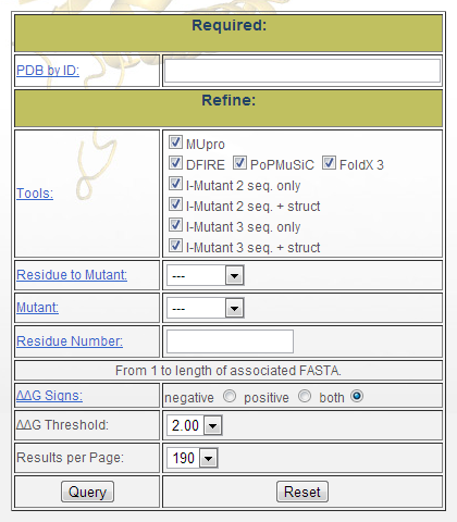
Figure 1: Database query form

• "PDB by ID": The first parameter is the Protein Data Bank (PDB) [1] code. Queries can only be made for one structure at a time to avoid someone requesting all the results contained in the database. Such a query would break the server and the user’s web browser. In the future, will we be supporting side-by-side comparison of two or three proteins.
  
• "Tools": The second parameter is a series of checkboxes that may be used to indicate which tool’s data should be displayed. 4+2+2 are available: DFIRE [2], MUpro [3], PoPMuSiC [4], and FoldX 3.0 beta 5.1 [5] + 2 versions of I-Mutant 2.0.6 [6] (one with the only sequence as input and the other one with sequence + structure data as input) + 2 versions of I-Mutant 3.0.6 [7] (as previous). A tool may be checked even if the database does not contain data for it, in this case the query will return no results.� By default, data for all tools will be returned.
  
• "Residue to Mutant": The third parameter concerns the mutation. One can choose which kind of amino acid (among the 20 possible ones) is of interest.
  
• "Mutant": One can also choose the amino acid that will be the mutant. Of course, the mutated amino acid must be different than the residue to mutate. By default, every residue among the sequence is represented with the 19 possible mutations.
  
• "Residue Number": The fifth parameter is the amino acid number. The numbering always begins from 1 and goes to the length of the primary sequence. It does not follow the PDB numbering. In case the user specifies a residue letter and a number, it will check if this is the right amino acid at this position. By default, no residue is specified and so all residues will be considered.
  
• "ΔΔG Sign": The sixth parameter offers the possibility to visualize only mutations which increase the stability or, opposite, which decrease the stability or even both changes (default mode).
• "ΔΔG Threshold": The seventh parameter allows the user to specific the magnitude of ΔΔG that should be considered. For instance, if 2.00 is selected, then any� |ΔΔG| values less than 2.00 will be assumed to be neutral and not be classified as stabilizing or destabilizing.
• "Results per Page": The last parameter offers the possibility to limit the number of results displayed on the result page. By default, the value is set to 190 lines which correspond to the results of all the 19 possible mutations for 2 residues and for all the tools. Even if the option is available, it is strongly advised not to select the "all" option especially for long proteins.
  

�

Results Visualization

Once data is available in the database, it can be visualized with three different methods.

Raw results
The first way of visualizing results is directly reading data extracted from the database. The user retrieves all the information contained in the database and relative to the query they submitted. There is no data post processing and it is the simplest way of getting the results. Figure 2 is an example of the results corresponding to a simple query with for the MUpro data for the 1asu protein.

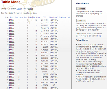
Figure 2: Raw results obtained for the 1asu protein

Eight columns are available:

• "Line": This is just a counter for the result line. It helps the user to find one important result after many scrolling and page changes.
  
• "Tool": In case the user does not specify a tool, its name is written here. When the user clicks on the name of the tool, he will directly be connected to the official Web site of the tool.
  
• "Res. Num": Residue number. As previously noted, the numbering index begins with 1. The PDB numbering is not applied here. The PDB numbering is not use here; instead we use the number from the corresponding FASTA sequence. Currently, if the FASTA sequence contains some X residue, then the numbering will exclude it, as if that residue does not exist. However, we feel this is less than optimal. Only MIR, TEF, and MUpro will process these filtered residues to give a sense of the data. Other tools will only run with unmodified indices.
  
• "Res. Letter": This corresponds to the native amino acid present in the sequence at the position given by the res. num index.
  
• "Mut. Letter": This is the mutation in which the native residue will be mutated. Res. letter and Mut. letter should always be different.
  
• "ΔΔG": This is the most valuable information in the database as it is the main result we get from each tool. Indeed, all the other fields (except "Stabilizing?", see below) are given as input and help to make the correspondence between these results and the submitted query. The unit is kcal/mol. A negative sign implies that the structure stability is increased by the mutation and conversely, a positive sign implies that the structure stability is decreased by the mutation.
  
• "Stabilizing?": This column summarizes the predicted effect of the mutation. The accuracy of this column is dependent on the tool being examined. It does not directly reflect the correct effect.� This field is here to quickly indicate whether the predicted value has a stabilizing effect or not. A YES corresponds to a negative ΔΔG, a NO is associated to a positive ΔΔG, and a NEUTRAL corresponds to ΔΔG magnitude less than the required threshold.
  
• "Protherm link": Protherm [8] is a database devoted to the storage of thermodynamical experimental data that has been produced and published in the scientific literature. There is not a lot of available experimental data for the proteins in the database. It is thus normal if most of the database entries do not give this information. When the user clicks on the Protherm link, they will be directed to the Protherm web site with the result page related to the considered mutation. We are working on better integrating these results into our Web site.

Right side menu:

• "3D mode": Clicking this button will open a new window that visualizes the protein in 3D.
• "2D mode": Clicking this button will open a new window that visualizes the protein with a 2D graph.
• "CSV file": Clicking the highlighted link will allow one to download the data in CSV format.
  

The user can sort the results by clicking on each of the column header. By default, the list is ordered by the residue number. Results are split into different pages to avoid scrolling a long list of information and the number of results per page can be changed in the query form. We recommend users use the CSV download if they need to manipulate or view large portions of the given data.

2D mode

This visualization mode is intended to quickly interpret the results for a given structure. In one graph, the user can superpose the results for any set of tools, they also have the ability to smooth the curves in order to have a clearer look. The user may display a consensus which is calculated as the mean of data provided by each tool. We also provide the results from the Most Interacting Residues (MIR) [9] prediction and the Tightened End Fragment (TEF) [10] assignment (if PDB is available). Figure 3 shows the pop-up that manage this functionality. Graphs are generated with the GNUplot [11] software.

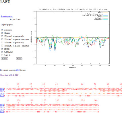
Figure 3: Pop-up of the 2D visualization mode. The graphs represent the stability score along the 1asu sequence

On the right is the graph. It represents the stability score of each amino acid along the sequence of a given structure. The stability score summarizes the effect of the 19 possible mutations for an amino acid. If a mutation has its ΔΔG with a negative sign of the required threshold (thus it increases the stability of the structure), we add +1 to the score. Conversely, if a mutation has its ΔΔG with a positive sign of the required threshold (thus it decreases the stability of the structure), we add -1 to the score. We repeat this operation for the 19 possible mutations on each amino acid and we finally obtain a score included in the range of [-19: +19]. Therefore, the use of the word stability actually concerns the stability after the mutation.

This kind of graph is useful to quickly visualize where are the regions in a sequence that are sensitive to mutations. Indeed, if almost every mutation has a destabilizing effect, the score will be around -19. Conversely, if almost every mutation has a stabilizing effect, the score will be around +19. The ability to distinguish these extrema is of great importance as it highlights the positions which are very sensitive and which, by the way, should play a role in the folding of the structure. We hope by this mean of adding the scores, to get rid of insignificant individual ΔΔG contributions. We recommend to focus mainly on maxima and minima of this curve, because the variations among individual tools may present diverging behaviors. Maxima and minima positions are often coherent among the various tools. This is a general trend, not a must. So interpretation should be the following: Positions close to -19 must be mutated with caution, while positions close to 19 are rather secure. This is the only conclusion one can retain from such a rough model.

The smoothing process is applicable as the original graphs are very sharp and it is difficult to evaluate them. Currently we smooth them with the Pascal triangle. This technique takes into account the neighborhood of a point (4 neighbors from each side of the point in this case) and thus reduces the number of peaks. The downside is the loss of accuracy but it helps to localize the regions of interest. This smoothing procedure is off at the origin of the peaked values at both ends of the curve, because some neighbors are missing for a complete triangle application. We think that much better smoothing of the ΔΔG values is possible and we plan to enhance this feature in the future.

In the scope of providing a meta server with information related to the folding core of proteins, we offer the possibility to get the MIR prediction and the TEF assignment of the studied protein. These two methods are summarized below and for further details, see the related references.

• MIR: A Monte Carlo algorithm is used to simulate the early steps of protein folding on a (2,1,0) lattice. An amino acid is randomly selected and displaced to a new available position on the lattice. The energy of both initial and final conformations is computed from the Miyazawa and Jernigan potential of mean force [12] and the Metropolis criterion is then applied [9, 10]. The starting point is the protein structure in a random coil conformation and the simulation is typically of 106 Monte Carlo steps.

This simulation is repeated 100 times with different initial conformations. The number of neighbors is recorded after each series of 10 Monte Carlo steps, and at the end of the process, an average Number of Contact Neighbors (NCN) is calculated for each amino acid of the sequence, at the exclusion of the first neighbors along the main chain. Amino acids surrounded by many others play a role in the compactness of the protein and thus are called Most Interacting Residues (MIR).

• TEF: Along the backbone of a protein, some pairs of amino acids can be very close in several places, with a typical distance between their alpha carbons below 10�. The histogram of the sequence separation between these "contact" amino acids is not smooth, and presents a maximum around 25 amino acids [13]. These sequence fragments were initially called closed loops [14].

Later on, it has been shown that the ends of these closed loops are mainly occupied by hydrophobic amino acids. A thorough analysis demonstrated that these hydrophobic amino acids were highly conserved among structures of the same family, although containing distantly related sequences: these positions were called topohydrophobic [15].

The concept of TEF emerged from the junction between closed loops and topohydrophobic positions.

Under the graphs, the protein sequence, the TEF assignment and the MIR prediction are displayed. We are looking into mapping zones of the graphs with this information to better localize the regions of interests.

3D mode

This mode is intended to aid structural biologists who are more accustomed at manipulating 3D structures and objects. The Jmol [16] 3D applet has been used in our project as its development has been targeted specifically for Web browser integration.

Several options are available like the ability to display the stability score computed for each amino acid with a selected tool. Please note that consensus data is not available here yet. A small sphere located on the alpha carbon of each amino acid coupled with a gradient of color displays this information. The color palette goes from red representing a score of -19 to blue for a score of +19. The user can also locate the TEFs assigned to the protein structure. In this case, the fragments are selected and the cartoon representation is colored in a different color for each TEF. When there is an overlapping between two TEFs, the resulting color of the overlap is a mix between the colors of the two TEFs. For example, if the first TEF is in blue and the second one in yellow, the overlap segment will be in green. The last option is the localization of the residues characterized as MIR. A transparent purple sphere with a greater diameter than the one for the stability score is represented on the alpha carbons of the MIR. Figure 4 shows an example of the 3D applet for the 1asu structure.

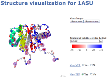
Figure 4: Pop-up of the 3D visualization mode for the 1asu structure. All the display options have been selected: stability score for the DFIRE tool, MIR prediction and the TEF assignment.

The Jmol applet is a powerful visualization software tool which offers many options. We only provide some predefined scripts we assume to be the best representation ways given the information. You may access all the Jmol options by right clicking inside the applet and selecting all the options you want. This may cause the loss of existing information. In this case, the user can reset the view by clicking the appropriate button. The raw structure button provides the display of the whole structure i.e. all the chains if several exist in a wireframe representation.

Submitting Jobs SPROUTS

The submission interface offers two basic ways to submit proteins for analysis. A user may submit a valid DPB ID and the server will automatically retrieve all needed data from the PDB. Alternatively, a user may submit custom data in FASTA format. In the latter case, the user will also be required to enter a 4-letter alphanumeric code to identify the submission and later retrieve the results from SPROUTS database and offered to submit their data in DSSP and/or PDB formats. A PDB ID or all three files (FASTA, DSSP and PDB) must be submitted to execute the complete workflow. Figure 5 is a snapshot from the page and shows the main options available to the user. The first part of the form allows the user to select the source of data to use while the second part requires the user to enter an email address so they can be notified at the completion of the request.

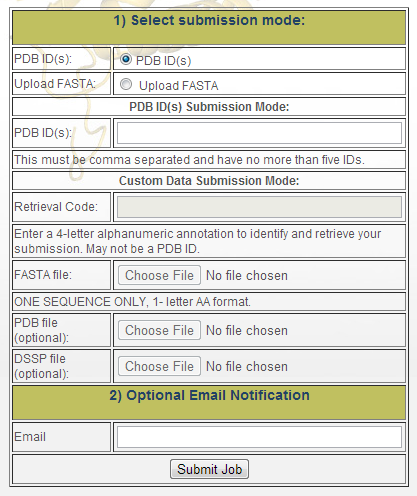
There are two data sources:

• "PDB ID(s)": Here the user may enter Protein Data Bank (PDB) [1] IDs for automatic analysis. Up to five PDB IDs may be entered here, provided that they are separated by commas. When a PDB ID that is valid (exists in the PDB) and not in the database is submitted, it will be queued within a hour If there is an issue with any of the submitted PDBs, the user will be notified by the page following submission. Note that proteins longer than 500 residues cannot be run automatically on the workflow. If you are interested in running longer proteins, please contact us.
• "Retrieval Code": Initially, the user must provide a retrieval that will be used to track the protein in our system. This must be a four letter alphanumeric string that is not a valid PDB ID. Based on the data that is provided to this form, the appropriate tools will be run. Proteins submitted this way will not be displayed on the auto-complete on the query page. Hence, the user must remember the code they have selected in order to retrieve its data or save the link provided on the following page.
• "FASTA file": The user must browse and select a text FASTA file from their local computer.� The FASTA file must contain exactly one sequence and contain the protein in the 1-letter AA format.�
• "PDB file" and "DSSP" file: optionally the user may browse for and select PDB and DSSP files to associate with their submission. For all input data, we analyze only chain A.
• "Email:" Optionally the user may enter an email to receive a notification with the retrieval code when the submission has been added to the queue and when it is processed. The email will not be used for any other process.
  

Conclusion

The initial project was a comparison of several tools devoted to the prediction of stability changes upon single point mutations on a given structure. The amount of produced data has given rise to the idea that these information should also benefit to other scientists that may be interested in. The decision of creating such a database was then on its way and after some discussions, the desire to offer more services than a data repository has emerged.

From the original 10 structures, we now have 129 structures with related results for the five mentioned tools. We also offer two modes to better interpret and analyze them in a more friendly way by graphs representation and by 3D structures with annotations for scientists more involved and accustomed to structural bioinformatics.

Our efforts are still underway to further propose more functions in order to increase the different levels of analysis. Another aspect will be to add other kind of data which might be related and thus we aim at proposing a non exhaustive but complete meta server on the protein folding core theme based on the protein stability.

OPTION DESCRIPTIONS

PDB ID: PDB ID of the query structure. This list represents all the structures that have been computed the possible tools.

Tool: List of the tools used to predict the stability changes upon point mutations. 4+2+2 are available: DFIRE [2], MUpro [3], PoPMuSiC [4], and FoldX 3.0 beta 5.1 [5] + 2 versions of I-Mutant 2.0.6 [6] (one with the only sequence as input and the other one with sequence + structure data as input) + 2 versions of I-Mutant 3.0.6 [7] (as previous). The two modes of I-Mutant are considered as two distinct tools as they do not use the same input.

Residue letter: The user can select from which type of residues he wants to get the results. The list contains the 20 different amino acids. In the results page, the one letter code will be used.

Residue number: The result selection can also be executed on the residue number in the protein sequence. For this purpose, the user has to enter a valid positive integer number. The numbering follows the sequence indices thus it always begins by 1 to n. The PDB numbering is not used here.

DDG Signs: ΔΔG gives information about the increase in stability or not for a given structure after a mutation has been applied. The user can choose to filter mutations at a high level based on their sign with this selection.

DDG Threshold: The user can choose to filter mutations by magnitude of ΔΔG that should be considered. For instance, if 2.00 is selected, then any� |ΔΔG| values less than 2.00 will be assumed to be neutral and not be classified as stabilizing or destabilizing.

Mutation letter: The user can select from which type of mutation he wants to get the results. The list contains the 20 different amino acids to substitute with the wild one. In the results page, the one letter code will be used.

SEQ: Protein sequence of the current structure. The 20 amino letter code is used and non standard amino acids are represented by the 'X' letter.

Smooth graphs: The smoothing process is relevant as original graphs are very sharp and it is difficult to evaluate them. We have decided to smooth them with the Pascal triangle. This technique takes into account the neighbourhood of a point (4 neighbours from each side of the point in this case) and thus reduces the number of peaks. The counterpart is the loss of accuracy but it helps to localize the regions of interest.

Gradient of stability score: One can represent stability score of each amino acid of a given protein and for a specific tool with a colored sphere located on the alpha carbon of the residue. A gradient from red to blue is used respectively representing the [-19:+19] score range. Normally, the five tools are available + the consensus which average the results of the five tools for each residue thus resulting in mean stability score values. If the query is tool specific, only the given tool can be selected. If the query is residue specific, all the gradients will be disabled and we suggest the user to refer to the table results. In case of missing residues in the structure file or exception errors for a given tool, the gradient is not available as the stability depends on the whole protein. Only the tools providing results for all the residue mutations are taken into account

View MIR: A Monte Carlo algorithm is used to simulate the early steps of protein folding on a (2,1,0) lattice. An amino acid is randomly selected and displaced to a new available position on the lattice. The energy of both initial and final conformations is computed from the Miyazawa and Jernigan potential of mean force [Miyazawa and Jernigan, 1996] and the Metropolis criterion is then applied [Papandreou et al., 2004; Chomilier et al., 2004]. The starting point is the protein structure in a random coil conformation and the simulation is typically of 106 Monte Carlo steps.

This simulation is repeated 100 times with different initial conformations. The number of neighbors is recorded after each series of 10 Monte Carlo steps, and at the end of the process, an average Number of Contact Neighbors (NCN) is calculated for each amino acid of the sequence. Actually, amino acids surrounded by many others play a role in the compactness of the protein and thus are called Most Interacting Residues (MIR).

View TEF: Along the backbone of a protein, some pairs of amino acids can be very close in several places, with a typical distance between their alpha carbons below 10�. The histogram of the sequence separation between these "contact" amino acids is not smooth, and presents a maximum around 25 amino acids [Berezovsky et al., 2000]. These sequence fragments were initially called closed loops [Ittah and Haas, 1995].

Later on, it has been shown that the ends of these closed loops are mainly occupied by hydrophobic amino acids. A thorough analysis demonstrated that these hydrophobic amino acids were highly conserved among structures of the same family, although containing distantly related sequences: these positions were called topohydrophobic [Poupon and Mornon, 1998].

The concept of TEF emerged from the junction between closed loops and topohydrophobic positions.

References

1. Berman, H.M., Westbrook, J., Feng, Z., Gilliland, G., Bhat, T.N., Weissig, H., Shindyalov, I.N. and Bourne, P.E. (2000) The Protein Data Bank. Nucleic Acids Res., 28, 235-242.
2. Zhou, H. and Zhou, Y. (2002) Distance-scaled, finite ideal-gas reference state improves structure derived potentials of mean force for structure selection and stability prediction. Protein Sci., 11, 2714-2726.
   
3. Cheng, J., Randall, A. and Baldi, P. (2006) Prediction of protein stability changes for single site mutations using support vector machines. Proteins, 62, 1125-1132.
   
4. Gilis, D. and Rooman, M. (2000) PoPMuSiC, an algorithm for predicting protein mutant stability changes: Application to prion proteins. Protein Eng., 13, 849-856.
   
5. Guerois, R., Nielsen, J. E. and Serrano, L. (2002) Predicting changes in the stability of proteins and protein complexes: a study of more than 1000 mutations. J. Mol. Biol., 320(2), 369-387.
   
6. Capriotti, E., Fariselli, P. and Casadio, R. (2005) I-Mutant2.0: predicting stability changes upon mutation from the protein sequence or structure. Nucleic Acids Res., 33, W306–W310.
   
7. Capriotti, E., Fariselli P, Rossi, I. and Casadio, R. (2008) A three-state prediction of single point mutations on protein stability changes. BMC Bioinf., 9(Suppl 2), S6.
   
8. Kumar, M.D., Bava, K.A., Gromiha, M.M., Prabakaran, P., Kitajima, K., Uedaira, H. and Sarai, A. (2006) ProTherm and ProNIT: thermodynamic databases for proteins and protein-nucleic acid interactions. Nucleic Acids Res., 34, D204-D206.
   
9. Papandreou, N., Berezovsky, I.N., Lopes, A., Eliopoulos, E. and Chomilier, J. (2004) Universal positions in globular proteins. Eur. J. Biochem., 271, 4762-4768.
   
10. Chomilier, J., Lamarine, M., Mornon, J.-P., Torres, J.H., Eliopoulos, E. and Papandreou, N. (2004) Analysis of fragments induced by simulated lattice protein folding. C R Biol., 327, 431-443.
    
11. The gnuplot Team. (2012) gnuplot: a portable command-line driven graphing utility. http://www.gnuplot.info
12. Miyazawa, S., Jernigan, R.L. (1996) Residue- residue potential with a favorable contact pair term and an unfavorable high packing density term for simulation and threading. J. Mol. Biol., 256M, 623-644.
    
13. Berezovsky, I.N., Grosberg, A.Y. and Trifonov, E.N. (2000) Closed loops of nearly standard size: common basic element of protein structure. FEBS Lett., 466, 283-286.
    
14. Ittah, V. and Haas, E. (1995) Nonlocal interactions stabilize long range loops in the initial folding intermediates of reduced bovine pancreatic trypsin inhibitor. Biochem., 34, 4493-4506.
    
15. Poupon, A. and Mornon, J.P. (1998) Populations of hydrophobic amino acids within protein globular domains: identification of conserved "topohydrophobic" positions. Proteins, 33, 329-342.
    
16. The Jmol Team. (2012) Jmol: an open-source Java viewer for chemical structures in 3D. http://www.jmol.org